Eucalyptus nitens, recovery and economics of processing 15 year old trees for solid timber

Report Date: May 2015

Author: Dean Satchell, Sustainable Forest Solutions, R.D. 1 Kerikeri, Northland 0294
+64 21 2357554

Appendix 1: Assumptions in Discounted Cash Flow Analysis
Appendix 2: Sawn timber price estimates
Appendix 3: Literature review - Value-based survey pricing methods
Appendix 4: Literature review - Estimating profitability of growing E. nitens for solid timber production
Appendix 5: Sawmilling method
Appendix 6: Flooring price survey instrument
Appendix 7: Survey results table
Appendix 8: Survey analysis
Appendix 9: Wood physical properties, test results
Appendix 10: Glossary of terms
Appendix 11: Case study stand plot
Appendix 12: Comparison between levels of internal and surface checking
Appendix 13: Air drying experiment
Appendix 14: Sensitivity analysis

• Photo Gallery »
• Treegrower Article »
• Thesis »

---

Methods

1. Pricing of flooring timber

 

Introduction

A market survey of merchants and flooring timber specialists was undertaken to produce price estimates for the flooring product profiles produced in this study.

Product profiles are the combination of characteristic levels that make up a graded piece of timber to price. For this study between species quality characteristics are categorised as appearance, hardness and movement in service, whereas within species quality characteristics are categorised as board width, grade and length.

Pricing of graded E. nitens product profiles was based on a reference product with price adjustments by survey respondents for each characteristic level that varied from those of the reference product. The reference price was the wholesale price for the reference profile of the reference species.

Flooring timber reference product = reference profile for the reference species
Flooring timber comparison product = reference profile for comparison species

Flooring Timber Reference Species

The reference species was selected as Victorian ash because this is the species most similar to E. nitens in terms of quality characteristics. Victorian ash was considered by all interviewees to be the species most similar to E. nitens in terms of quality characteristics.

The comparison species was E. nitens.

Reference species = Victorian ash (imported from Australia).
Comparison species = E. nitens

Quality Characteristics of Flooring Timber

Quality characteristics were categorised into two groups:

• Between-species qualities.
• Within-species qualities.

Within-species quality characteristics each come in levels. Although discounts or premiums are measurable for grade and width levels for flooring timber species established in the marketplace, levels for board lengths and price discounts/premiums for these are neither implicitly nor explicitly available from available market prices.

Between-species quality characteristics such as hardness and movement in service are measurable, but appearance is subjective and evaluating discounts or premiums between species may not accurately reflect price in the market for the product. A market survey instrument offers the vehicle to empirically compare the appearance of a new timber species with an existing species and consequently price this as a quality characteristic.

Between-species quality characteristics

Between-species quality characteristic categories were appearance, hardness, and movement in service.

Within-species quality characteristics

Within-species quality characteristic categories were board width, board length, and board grade.

Other quality characteristics

Non-physical quality characteristics perceived by interviewees as influencing price were:

• Reputation;
• local vs imported timber products;
• sustainably produced vs non-sustainably produced timber, and
• plantation vs natural forest sourced timber.

Flooring Timber Reference Product

Wholesale prices landed in New Zealand could only be obtained for one grade and width for Australian sourced Victorian ash as a confirmed price landed in New Zealand. This species is only available as long-lengths for solid timber flooring product in New Zealand.

Flooring timber product reference profile = 108 mm x 19 mm width (nominal 125 mm x 25 mm width), Select grade, >1.2 m length.

Flooring timber reference product = reference profile for reference species
Flooring timber comparison product = reference profile for comparison species

Flooring timber reference product price = $4.09 per lineal metre at 10 June 2014

Estimating Utility for Quality Characteristics using survey methods

The survey took place in September 2014.

Two social survey methods were employed in a market survey to price quality characteristics and utility for the E. nitens flooring products produced in this case study, described in this methods section:

1. Dollar metric pricing of utility and part worth utilities using the graded-pairs comparison approach.
2. Constant-sum allocation pricing of part-worth utilities.

Both methods are self-explicated stated preference approaches that directly estimate utilities for the product profile as described below.

Twenty-seven respondents were selected for participating in the market survey. These individuals represented the population of flooring timber experts and companies currently in business in New Zealand, including floor layers, timber flooring retailers and timber flooring wholesalers. 

Survey respondents were each made aware of the different attributes they were to judge before evaluations commenced.

The survey instrument was web-based and used check boxes, fields and photographic images to induce responses (Appendix 6: Flooring price survey instrument). Impartial guidance was provided via telephone during each survey interview to ensure respondents understood each question and how to answer it.

Discounts and premiums were quantified for each between-species characteristic to determine the price for the E. nitens reference product with the same product profile as the reference species.
For each E. nitens product profile to be priced, discounts and premiums for each quality characteristic were summed for a discount or premium for the profile.

Pricing of timber profiles

Pricing of the timber profiles used a three-stage approach:

1. The between-species premium or discount for the comparison species (E. nitens) was estimated as the averaged respondents’ discount or premium from the reference product (Victorian ash) to make the reference profile for the two species to be of equal worth. This discount or premium adjusted the price for the E. nitens reference profile from the reference product price. Then,
2. the price discount or premium for each level of each within-species quality characteristic was estimated as the averaged respondents’ price discount or premium to make the two levels of each characteristic being compared of equal worth.
3. Each discount or premium was quantified as a monetary value by multiplying the E. nitens reference price by the percentage discount or premium where the level of the characteristic differed from the reference profile. Discounts and premiums were then summed for the price of each product profile.

Graded-pairs Survey Method

Between-Species Evaluations

Respondents judged the total utility of E. nitens as a dollar metric by comparing appearance, hardness and movement in service between E. nitens and Victorian ash, given a price for Victorian ash. This was converted to a percentage discount or premium after averaging between respondents.

Within-Species Comparisons

Although respondents judged levels of each quality characteristic independently of other quality characteristics, they were asked to consider the quality characteristics as a bundle when evaluating each characteristic’s part-worths.

Board grades

Three levels of board grades were presented to respondents as photographic images each representing floors:

• Grade 1 (representing both FFT Clears and AS Select grades) - the reference product grade.
• Grade 2 (representing both FFT Standard and AS Standard grades).
• Grade 3 (representing both FFT Feature and AS High Feature grades).

Two grades were compared at a time:

• Grade 1 with Grade 2, and
• Grade 1 with Grade 3.

For each comparison, respondents estimated the percentage discount or premium they would allow for the second grade from the first grade for the two grades to be of equal worth. The discounts and premiums were averaged between all respondents for each comparison. A monetary discount or premium for each grade level where different to that of the reference profile was calculated by multiplying the comparison product’s price by the percentage discount or premium for that level. This discount or premium was respectively subtracted or added to the comparison product’s price for the resulting price of each grade where the width and length was the same as the reference profile.

No distinction in price was made between FFT Over Joists and FFT Overlay grades.

Board widths

For board widths three nominal levels were presented to respondents:

• 150 mm;
• 125 mm (The reference profile width); and
• 100 mm.

Two widths were compared at a time:

• Nominal 150 mm board width per square metre of floor was compared with nominal 100 mm board width per square metre of floor, and
• nominal 150 mm board width per square metre of floor was compared with nominal 125 mm board width per square metre of floor.

For each comparison, the respondent estimated the percentage discount or premium they would allow for the second width from the first width for the two widths to be of equal worth per square metre. These discounts and premiums were averaged between all respondents for each comparison. Discounts or premiums for each level were then converted to a lineal metre rate for each width. Prices for widths were then calculated for each grade by multiplying the grade price by the discount or premium for each width. This monetary discount or premium was respectively subtracted or added to the price of each grade for the width prices for each grade where length was the same as the reference profile.

Board lengths

Discounts for boards shorter than 1.2 m (i.e. shorter than the reference profile length) were applied as two categories:

• 30 cm - 60 cm lengths as end-jointed product, and
• 60 cm - 120 cm lengths as end-matched product.

Board lengths 30 - 60 cm

For pricing the 30 - 60 cm board lengths, respondents were each asked to evaluate photographic images of a strip floor made from 30 - 60 cm board lengths and compare this with a floor made from boards of the same width but from random lengths greater than 1.2 m (the reference profile length). Respondents were informed that the product being compared was edge-jointed long-length flooring product made from lengths between 30 cm and 60 cm. Comparisons of worth were made per lineal metre, based on the appearance of the floor being compared. Respondents were also asked to consider that the jointed product was available in long lengths when comparing worth.

For this comparison, respondent’s each estimated the percentage discount or premium they would allow for the short length category from the long length category for the two to be of equal worth. This discount was averaged between all respondents for the comparison. Monetary discount for the shorter length was calculated by multiplying the price for each grade and width combination by the discount or premium applicable to that length. For the 30 - 60 cm category, the discount was then subtracted from the price for the > 1.2 m category for each grade and width combination.

Boards were then discounted further by the cost per lineal metre for edge-jointing for a residual product value for each profile with 30 - 60 cm lengths.

Board lengths 60 cm - 120 cm

Boards in the end-matched category were discounted only by the cost per lineal metre for end-matching these boards. Price for 0.6 m - 1.2 m lengths compared with >1.2 m lengths were not directly estimated by respondents. Instead, it was assumed that the appearance of a floor laid from 0.6 m - 1.2 m lengths would not attract a lower price than a floor laid from > 1.2 m lengths and that costs for installation would not vary for the two timber lengths.

The additional cost of end-matching was subtracted per lineal metre from the >1.2 m category price for a residual product value for profiles with 0.6 m - 1.2 m lengths.

Price results are in Appendix 2: Sawn timber prices.

Constant Sum allocation survey method

Between-Species Evaluations

Respondents were asked to weight importance of between-species quality characteristics. A constant sum of 100 was used to allocate the relative importance of the three between-species quality characteristics (appearance, hardness and movement in service) to provide trade-offs between these attributes.

Respondents were asked to rate desirability of each level of the hardness attribute on a scale of 1 - 10. Janka Hardness (kN) levels provided were:

• Very hard (9 +).
• Hard (7 - 8).
• Medium hardness (5 - 6).
• Soft (4 - 5).
• Very soft (3 - 4).

Respondents were asked to select 10 for their most desirable hardness level and then rate the others comparatively.

Respondents were asked to rate desirability of each level of the movement in service attribute on a scale of 1 - 10. Movement in service levels provided were:

• Small levels of movement (< 3.0 %).
• Medium levels of movement (3.0 - 4.5 %).
• Large levels of movement (> 4.5 %).

Respondents were asked to select 10 for their most desirable movement level and then rate the others comparatively.

Appearance was assessed for desirability by rating photographic images portraying a floor of the same grade and width for both species. Rating was on a scale of 1-10 and respondents were asked to rate their most desirable species at 10.

Part-worth for hardness

The individual respondent’s desirability rating for the category corresponding to the janka hardness test result for each of the two species being compared (the reference species Victorian ash and the comparison species E. nitens) was then multiplied by the importance weight that the respondent allocated for hardness, revealing the individual respondent’s hardness part-worth value for each species.

Part-worth for movement in service

The individual respondent’s desirability rating for the category corresponding to the long term movement in service test result level for each of the two species being compared (the reference species Victorian ash and the comparison species E. nitens) was then multiplied by the importance weight that the respondent allocated for movement in service, revealing the individual respondent’s movement in service part-worth value for each species.

Part-worth for appearance

The part-worth value for the appearance characteristic was determined by multiplying the individual respondent’s desirability rating for each species by the importance weight the respondent allocated for appearance.

Total-worth for species

The individual respondent’s part worth’s for each quality characteristic were summed, then averaged for all respondents for each species as overall utility for each species. The overall utility for the comparison species (E. nitens) was then converted to a percentage discount based on the ratio between overall utility for E. nitens and overall utility for the reference species (Victorian ash). The monetary discount for the comparison species from the reference species was then calculated by multiplying the price for the reference species by the discount percentage. Price of the comparison species for the reference product profile (length > 1.2 m, width 125 mm nominal, select grade) was then calculated by subtracting the discount from the price of the reference product (the reference species and reference profile).

Within-Species Evaluations

Respondents were asked to weight within-species quality characteristics. A constant sum of 100 was used to allocate the relative importance of the three between-species quality characteristics (grade, width and length) to provide trade-offs between these attributes.

Respondents rated desirability of each level of the length attribute on a scale of 1 - 10. Length levels provided were:

• > 1200 mm.
• 600 - 1200 mm.
• 300 - 600 mm.

Respondents were asked to select 10 for their most desirable length level and then rate the other levels comparatively.

Respondents rated desirability of each level of the width attribute on a scale of 1 - 10. Nominal width levels provided were:

• 150 mm.
• 125 mm.
• 100 mm.

Respondents were asked to select 10 for their most desirable width level and then rate the other levels comparatively.

Grade was assessed for desirability by rating photographic images portraying a floor of each grade. Grades provided were:

• Select/clears grade (low levels of natural feature).
• Standard grade (some natural feature).
• High feature/feature grade (high levels of natural feature).

Rating was on a scale of 1 - 10 with respondents asked to rate their most desirable grade at 10 and then rate the other grades comparatively.

Part-worths for levels of quality characteristics

Utility was estimated for each level of the quality characteristics.

Each quality characteristic’s importance weight was multiplied by the desirability rating for each level of the characteristic to produce the respondent’s part-worth utility that level of the quality characteristic.

Total-worths for product profiles

A product’s utility is made up from part-worth utilities for the levels of characteristics that comprise the products profile.

Total worth for each product profile was calculated for each respondent as the sum of part-worths for the characteristic levels specified in that profile. Overall utility for each product profile was calculated by averaging overall utility from each respondent for the profile.

Utility for each profile was then converted to a percentage discount or premium based on the ratio between overall utility for the profile and overall utility for the reference profile. The monetary discount or premium for the profile from the reference profile was then calculated by multiplying the price for the comparison species reference profile by the percentage discount or premium. Price for each comparison product profile was calculated by subtracting the monetary discount from the price of the comparison species reference profile.

No distinction in price was made between FFT Over Joists and FFT Overlay grades.

Pricing Methods - 50 mm and 75 mm Wide Boards

50 mm and 75 mm wide boards were graded to FFT Panel Laminating or FFT Joinery grades:

• FFT Panel Laminating clear one face,
• FFT Panel Laminating clear two faces, or
• FFT Joinery clear four faces.

Two test panels were glue-laminated from the 75 mm material at A&J Wang Christchurch. One panel was constructed to 3.0 m length and made from full-length boards graded to clear one face. The panel was constructed with the graded clear edge upward and the best ends to one end of the panel. The other panel was 3.0 m long and made by butt-joining short board lengths graded to clear one face. These two types of material produced two different quality panels for pricing.

Costs for preparing and laminating the panels were quantified for each panel.

The panels were sold to determine market prices for the two panel products, each of different quality.

Board prices were calculated as a residual value by subtracting costs from sale price and converting net revenue to a per-lineal metre for the input timber product.

Price results are in Appendix 2: Sawn timber prices

Intangible quality characteristics

In consultation with timber market specialists, additional intangible quality characteristics identified as influencing price were included in the survey as characteristics for respondents to price. Respondents were asked to value the worth of:

• Reputation for quality (species) as a price discount for a new species such that they would prefer to buy this species compared to a species with an established reputation for quality.
• Price premium for locally produced product (if any) that respondents would pay, compared with an imported product of equivalent quality.
• Premium for sustainably produced timber (if any) that respondents would pay, compared with a timber that held no sustainability credentials.
• Price premium for plantation timber (if any) that respondents would pay, compared with timber extracted from natural forests.

These premiums and discounts were each averaged between respondents and were then summed and used to adjust E. nitens product prices for the purposes of a sensitivity analysis. E. nitens was classified as:

• Reputation for quality = New species to the market
• Local product = yes
• Sustainably produced product = yes
• Plantation timber = yes

E. nitens and Victorian ash physical properties

Hardness

A single board sample of 50 cm length was cut from the middle section of a randomly selected blanked nominal 125 mm board from each E. nitens log sawn in this study.
Six samples of nominal 125 mm wide and 25 mm thick quartersawn Victorian ash were randomly selected from stock that a merchant (Timspec Auckland) imported from ASH, Victoria, Australia during 2014.

All samples were sent to Scion Rotorua and were tested for the following physical properties:

• Density,
• hardness, and
• movement in service.

Samples were all tested twice on one face for Janka hardness and these results averaged.  The hardness quantity result for both species was incorporating into the survey questions that determined between-species prices.

Movement in service

All samples were tested for long-term dimensional stability. Long-term movement is expressed as the percentage of movement occurring across the width of the board when the moisture content changes from equilibrium at 85% RH to equilibrium at 35% RH.

Samples were prepared into test samples that were 70 mm wide, 50 mm long and 10 mm thick. Long-term movement was assessed by equalising standard sized samples in conditions of 25°C and 85% relative humidity. When the samples were at equilibrium (determined by having a stable mass) the samples were weighed and width and length were measured. The samples were then exposed to conditions of 25°C and 35% relative humidity. When the samples again reached equilibrium they were weighed and the width and length remeasured. The difference between the two width measurements was calculated as a percentage of the width in the 35% humidity conditions. The classification system categorises sum of radial and tangential movements as:

• Small <3.0 %
• Medium 3.0 – 4.5 %
• Large >4.5 %

Results were incorporated for both species into the survey questions that determined between-species prices.

Density

Density was measured for all samples at test by weighing a sample cut from the test piece immediately after testing for hardness. The sample was oven dried at a temperature of 103 degrees Celsius until the weight was constant. The samples were weighed again and the weight loss was divided by the final oven dry weight and expressed as percentage moisture content for the test samples at test.

 

---

2. Production methods

 

Introduction

 

Methods for processing logs into sawn product were required that minimised degrade, minimised costs and maximised grade recoveries to represent current industry best practice in converting E. nitens logs into profiled timber products. Prices for grade profiles were required in order to estimate sawn timber revenue for each sample log, as were detailed costs for each production process.

Case Study Trees

The case study comprised a small stand of 55 E. nitens trees that were planted by farm forester Patrick Milne near Rangiora on a reasonably well drained but moist fertile Canterbury plains site exposed to the west. These trees were planted at a 3 m x 3 m spacing and were pruned and thinned in expectation of solid timber production. The trees were 15 years old at harvest. All trees in the case study stand were measured for diameter at breast height (DBH) and height. Height measurements were recorded with a vertex III hypsometer. The stand was also mapped as a scale diagram to document the exact position of each tree in the stand, which were in two distinct areas (see Appendix 11).

Inventory and sample plots

Because the case study stand was not a contiguous area of trees, two plots, each 28 m x 8 m, were placed on the scale diagram to avoid edge trees and to provide plots that held representative stockings for a larger hypothetical stand (Appendix 11). An inventory of tree heights and tree diameters at breast height over bark (DBHOB) was produced from these two plots. Values for the two plots were averaged.

A Volume and Taper Equation for New Zealand Grown Eucalyptus nitens (Gordon, Hay, & Milne, 1990) provided volume and taper equations used for estimating plot log volumes, stem volumes and estimates of log SEDs. Log volumes and diameters were estimated from 0.3 m upward based on 3 m log lengths.

Logs were allocated to categories according to small-end diameter under bark (SEDUB):

• Waste = 0-10cm;
• pulp logs = 10-25cm; and
• sawlogs > 25cm.

Logs 1 and 2 from every tree were also classified as 'pruned buttlog'. Logs above 3 were classed as 'unpruned headlog'.  
Average plot tree numbers were scaled to a per hectare value, along with basal area, stem volumes, average diameters (DBHOB).

Case study logs

Trees were harvested and milled during November and December 2012. Trees harvested for sawmilling were selected to avoid edge trees and to represent the range of diameters present inside the stand. The other selection criteria requested by the owner was to production thin in order to evenly open up the stand and encourage further growth in remaining trees. This did not involve any specific selection criteria except that trees were harvested from throughout the stand and represented the full range of diamaters. Trees were harvested manually using a chainsaw and logs were immediately cross cut to 3 m lengths. Tree and log position numbers were marked on the logs and these were loaded onto a self-loading truck. Each of three log loads were weighed at a weighbridge and gross weight recorded. The empty truck was also weighed and total log weight calculated. Log specifications were to cross cut to a small end diameter of 25cm, however these were in most cases cut to 30 cm. Trees were reported as pruned to approximately 6.5 m, therefore the first two logs were classified as pruned buttlogs and above log two were classified as unpruned headlogs. No more than five logs were extracted from any one tree. Eight trees were harvested from which thirty two sample logs were milled.

Each log was painted on both ends with a base colour to represent the tree. Log positions were represented with a matrix of dots painted over the base colour with different colours representing each log position.

Logs were not debarked prior to sawmilling. The ends of each log were measured soon after cross cutting. Due to the oval nature of many of the logs, diameter was measured twice at each end from two perpendicular positions. These two measurements were averaged to produce an estimate for each end diameter. The log volume was then estimated using Smalian’s formula.

Individual sample log volumes were summed for a total sample log volume.

Volumes and weights

Tare was deducted from gross weight of each truckload and net weights were summed for total weight of sawlogs.

Total volume for logs was calculated by summing the volume of each log. Average green density per log cubic metre was calculated by dividing total weight for the logs by their total volume.

Slabwood was reloaded on the truck after sawmilling was completed and this was weighed four days after completion of sawmilling.

Board green weight was calculated by multiplying board green volume by weight per cubic metre.

Sawdust weight was assumed to be the difference between total weight and board weight plus slabwood weight.

Sawmilling

All logs were milled within five days of harvesting. This time frame was considered to be adequate to minimise defect in boards caused by end splits, but realistic for operational implementation. Although end-splits became evident on log ends over this time these were not severe in any logs.

Sawmilling took place on 29 November 2012 to 2 December 2012.

All logs were milled using exactly the same pattern (See Appendix 5). Slabbing was undertaken with a Woodmizer LT 40 horizontal bandsaw with a 3mm kerf. Logs were first cut through the pith after raising the log small end so the pith was parallel with the bed. Where necessary, measurements were taken from the bed to ensure the pith was level before making the first cut. Immediately after the first cut was made, measurements of deflection were taken at each end of the log and averaged. The log was kept intact and the two halves together turned 90 degrees. Again the small end was raised so the pith was level with the bed. The log was then slabbed at 28 mm thickness with each pair of slabs removed from the log on the return of the saw head. These dropped directly onto rollers that stockpiled slabs beside the Woodmizer twin-blade edger. Once approximately half of the log was removed as slabs, the two remaining cants were rotated 180 degrees and slabbed to the bed.

The Woodmizer twin blade edger operated simultaneously with the bandsaw for an efficient workflow so that as slabs were fed to the edger from the bandsaw these were edged. A separate operator ran the edger who both edged slabs and fillet stacked edged boards. Fillets were dry E. nitens with a thickness of 19mm and width of 25mm. Seven fillets were placed at 0.5m distances apart over each layer of boards and directly above the previous row of fillets, including at both ends of the stack. For each log the time it took to slab, from loading the log on to the bed to the completion of slabbing was measured in minutes. The stockpile of slabs waiting to be edged was observed to not increase during the slabbing process for each log and thus it was decided that recording the time the second operator was edging and stacking was not necessary, this being equal to the time recorded for slabbing.

Boards were edged to the following green widths:

Green sawn board widths

Nominal width (mm)	Green sawn width (mm)
150	165
125	133
100	108
75	83
50	57

 

Units of electricity and fuel were recorded per hour of operation along with prices for these (see Appendix 1).

Edging was based on judgement calls aimed at optimising value in preference to volume. This 'grade sawing' was undertaken by eye with no laser guidance. Slabs were first flipped and degrade was visually assessed on both faces prior to a decision on target board width and where to edge the slab for maximum value recovery. The pith was always removed and judgement calls were made on how much of the knotty core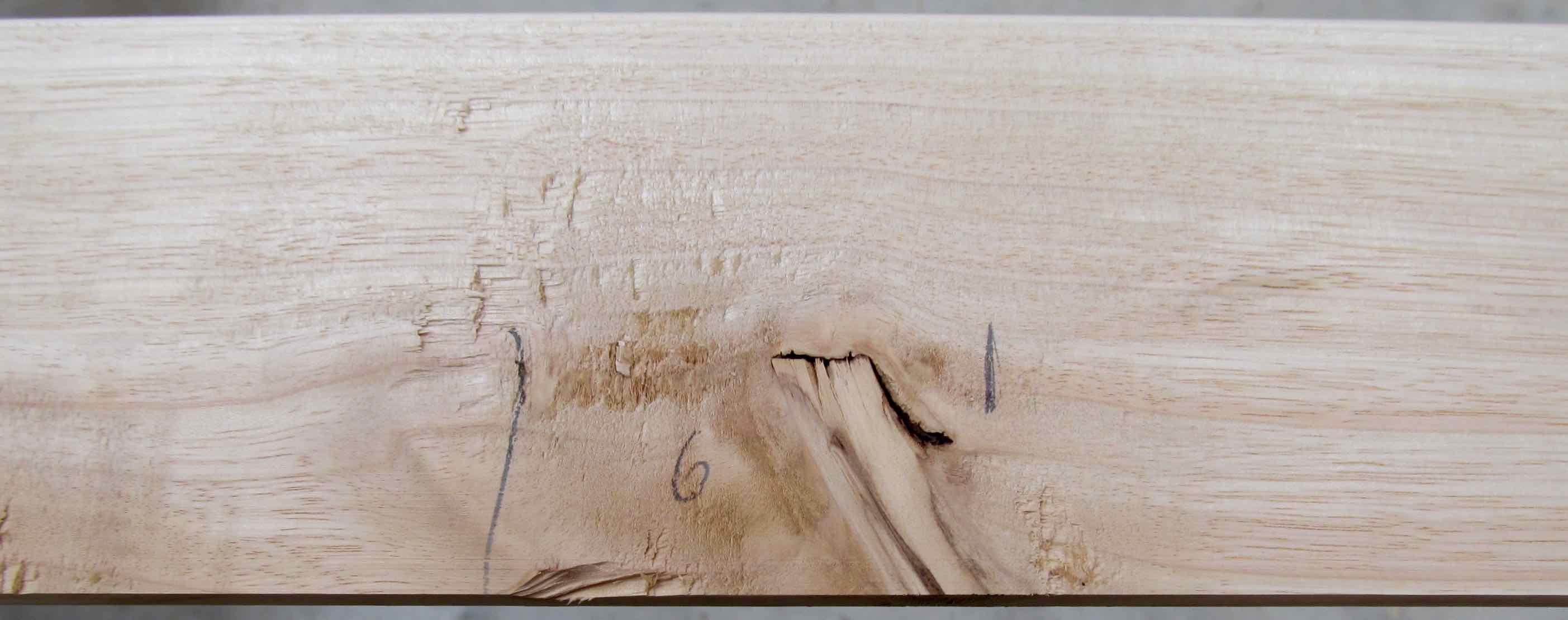
Pruning wound in the board. This will be docked with lengths of clearwood either side. would be removed. The edge closest to the periphery was usually removed as close to the periphery as possible. The Woodmizer twin-blade edger uses rollers to feed the slab through two circular saw blades, producing straight parallel edges at the width set by the operator. The slab is presented to the rollers freestyle with no fence for guidance.

The corewood was observed to have a contrasting colour to the surrounding sound wood when freshly sawn and was only present adjacent to the pith in quartersawn slabs containing central wood. In pruned logs this was always contained inside the pruning wounds. Unpruned logs had a corewood zone of similar size, but with knots extended outside of this. Where possible, corewood adjacent to the pith was edged out from slabs, regardless of whether the corewood was from pruned or unpruned logs.

Timber Drying

Fresh sawn boards were each randomly allocated to two treatments for the drying experiment (see Appendix 13).

Stacks were assembled on pallets designed for drying timber that provided airflow underneath, the first layer of sawn timber positioned 15cm from the ground or the stack below. 19 mm thick fillets were placed between layers at 50 cm intervals and at both ends of each layer.  The stacks were shifted by forklift immediately on completion of sawmilling.

Stacks were placed one on top of another in pairs, then wrapped with a single layer of microclima cloth, a semi-permeable white-coloured cloth used for reducing air flow through the stack. A single 1800 kg concrete slab was placed on top of each paired stack to weight it.

Stacks were air dried for 4 months. On April 20^th 2013 ten randomly selected boards on the outside of the stacks were measured for moisture content with a Trotec T500 Multi-board Measure Professional resistance method hand-held moisture-measuring instrument. This averaged 19.9% for the shed dried material and 18.73% for the yard dried material. Although it was decided the timber was dry enough to finish drying in the Solarola solar kiln at this point, because of unrelated production constraints the timber was not transferred into the kiln until 20 October 2013.  Both stacks were positioned in the kiln as a single charge. The timber stacks were removed from the kiln on 19 November and placed in a fully enclosed concrete floored shed used for storing dry timber.

Steam reconditioning was not performed on the timber.

Boards were measured for moisture content immediately prior to dressing (blanking and profiling) using a Trotec T500 Multi-board Measure Professional resistance method hand-held moisture-measuring instrument. Ten randomly selected boards from both stacks were tested for moisture content, which averaged 12.6%. This moisture content was deemed appropriate for dressing and grading the timber.

Timber Processing

The nominal 100 mm, 125 mm and 150 mm timber was dressed in two stages, blanking then profiling. Blanking took place on 20th and 21st November 2013 through a Logosol PH 260 four sider to 23 mm thickness and widths to the dimensions below.

Nominal and Dressed Board Widths

Board Nominal Width (mm)	Blanked Width (mm)	Profiled Width (mm)
150	155	128
125	125	109
100	96	83
75	72	- -
50	48	- -

 

All boards were dressed straight using a straight edge fence. Any crook was edged out by feeding boards through the machine with the concave edge against the fence, removing all crook at the risk of causing skip. Where crook was anticipated to be excessive and likely to result in loss of value as edge skip when profiled, the board was docked to provide shorter lengths for dressing straight. Where knots were observed to cause board distortion, the knot was docked out of the board prior to it being dressed.

Blanked boards of nominal sizes 100mm, 125mm and 150mm were dressed with a second pass into tongue and groove flooring profile at 19 mm thickness. Each blanked board was evaluated and a decision made on how to feed into the machine, based on levels of surface checking and collapse depth on both faces in an attempt to profile the best surface to the top (exposed) surface of the board. Where possible, excessive collapse or checking on the blanked board was turned down to the bottom face.

Blanked boards of nominal sizes 50mm and 75mm were not dressed further into profile.

Grading Procedure and Data Inventory

Grading was undertaken in February 2014. Boards were measured for moisture content immediately prior to grading using a Trotec T500 Multi-board Measure Professional resistance method hand-held moisture-measuring instrument. Ten randomly selected boards from both stacks were tested for moisture content, which averaged 11.75%.

Grading judgement calls took into account the value trade-off between predetermined value assumptions for grade and piece length (see Grading below). Board positions were marked where the board would be docked. Where possible timber was "docked" to achieve lengths that met equivalent grades under both sets of grading rules being employed.

For every board the following data was recorded:

• Board number;
• tree number;
• log number;
• drying treatment category;
• board nominal width;
• percentage of board length with checks present on the profiled surface;
• sum of length of checks present on the profiled surface; and
• end taper.

Individual boards were marked with a pencil into pieces, then each piece length measured and categorised. Each piece length was allocated to a grade or defect category. Grade and defect categories related to the width of the timber being graded and the grade rules being employed.

Grading

Grading of boards was undertaken using two sets of rules, Australian Standards AS 2796.2 – 2006 (AS) and Farm Forestry Timbers (FFT) grades as published in Grade Revision 1.1 October 2013.

Nominal 75 mm and 50 mm width boards were graded to Farm Forestry Timbers Standards but not to Australian Standards. Profiled nominal 100 mm, 125 mm and 150 mm board lengths were graded to both Australian Standards and Farm Forestry Timbers Standards.

Grading method was assumed to not influence price, with FFT Flooring clears grade holding the same value as AS select grade, FFT Flooring standard grade holding the same value as AS standard grade and FFT Flooring feature grade holding the same value as AS high feature grade.

Grading assumptions

Grading was undertaken based on the following assumptions:

• FFT Flooring overlay is worth 90% of FFT Flooring over-joist grade with the same length and width dimensions.
• Flooring product of 900mm - 1200 mm length is worth 90% of the price of >1200 mm flooring per lineal metre of the same grade and width.
• Flooring product of 600mm - 900mm length is worth 75% of the price of >1200 mm flooring per lineal metre of the same grade and width.
• Flooring product of 300 - 600 mm length is worth 25% of the price of >1200 mm flooring per lineal metre of the same grade and width.
• 125 mm flooring is worth 75% of the price of 150 mm flooring for the same grade and length.
• 100 mm flooring is worth 60% of the price of 150 mm flooring for the same grade and length.
• Standard grade is worth 80% of the price of select or clears grade of the same width and length.
• AS high feature grade is worth 50% of the price of AS select grade of the same width and length.
• FFT Flooring feature grade is worth 50% of the price of FFT Flooring clears grade of the same width and length.
• FFT Panel Laminating grade with length of 300 mm - 1500 mm is worth 50% of the price of >1500 mm length per lineal metre of the same width and grade.
• FFT Panel Laminating grade with four faces clear is worth the same by nominal volume as 150 mm wide FFT Flooring clears grade of the same length.
• FFT Panel Laminating grade with two faces/edges clear is worth 80% of the price of FFT Panel Laminating grade with four faces clear and of the same length and width.
• FFT Panel Laminating grade with one edge clear is worth 70% of the price of FFT Panel Laminating grade with four faces clear and of the same length and width.

Grading flooring product to Australian standards

Profiled nominal 100 mm, 125 mm and 150 mm width boards were graded to Australian Standards 2796.2 – 2006.

Defect categories for board pieces

Defect piece lengths were recorded in the following categories:

• End splits defect;
• box defect (Natural feature such as knots that do not meet grade requirements);
• collapse defect (skip);
• skip from wane;
• skip from cupping, twist);
• machining voids and want;
• excessive checks defect;
• tongue defect resulting from straightening out crook from boards;
• tongue defect resulting from collapse shrinkage; and
• piece length within each grade and length category combination.

Grade categories for board pieces

Graded piece lengths were recorded and categorised according to the following grades:

1. Select;
2. standard; and
3. high feature.

Piece length categories

Graded piece lengths were recorded in the following length categories:

• 300 mm – 600 mm;
• 600 mm – 1200 mm; and
• > 1200 mm.

Grading flooring product to Farm Forestry Timbers standards

Profiled nominal 100 mm, 125 mm and 150 mm width boards were graded to FFT Flooring grades as published in grade revision 1.1 October 2013.

Defect categories for board pieces

Defect piece lengths were recorded in the following categories:

• End splits defect;
• box defect (natural feature such as knots that do not meet grade requirements);
• collapse defect (skip);
• skip from wane;
• skip from cupping, twist;
• machining voids and want;
• excessive checks defect;
• grade category for each piece meeting a grade category (clears over joists, standard over joists, feature over joists, clears overlay, standard overlay, feature overlay); and
• piece length for each grade and length category.

Grade categories for board pieces

Graded piece lengths were recorded and categorised according to the following grades:

• Clears over joists;
• standard over joists;
• feature over joists;
• clears overlay;
• standard overlay; and
• feature overlay.

Piece length categories

Graded piece lengths were recorded in the following length categories:

• 300 mm – 600 mm;
• 600 mm – 1200 mm; and
• > 1200 mm.

Grading of 50 mm and 75 mm nominal width boards

Blanked nominal 75 mm and 50 mm width boards were graded to either FFT Panel Laminating grade as published in Grade revision 1.1 October 2013 or FFT Joinery grade as published in Grade revision 1.1 October 2013.

Grade estimates were made based on expected defect upon final profiling. Levels of checking and natural feature were not altered but skip was measured and an estimate was made of its expected presence or absence on the profiled surface. Sample boards were later dressed to profile immediately prior to laminating into panels because freshly planed surfaces were required for glue adhesion.

Grade interpretations and modifications

Concealed surfaces were graded to meet the structural conditions in both AS grades and FFT Over-joist grades.

Modifications to grade rules for the purposes of this study:

• AS select grade was downgraded to standard grade where checks were present.
• Box included clear short lengths under 30 cm.
• End splits included end checks.

Where wane or skip was present on concealed surfaces this was deemed acceptable provided it did not affect the stability of the boards or the tongue or groove connection.

Where two or more defects were present on a piece to be graded, defects held predetermined priorities.  The following category priorities applied:

• End taper held priority over end splits or any other defect.
• End splits held priority over box, skip and other defect.
• Box held priority over skip and excessive checks.
• Excessive checks held priority over collapse defect.

End taper was not categorised as defect, but instead was deducted from green sawn timber recovery and board lengths to be graded. Where end taper could not be distinguished from skip caused by collapse, a judgment call was made and one category selected. Where end taper could not be distinguished from taper caused by machining out crook, a judgment call was made and one category selected.

Where structural requirements for AS grades were not met on concealed surfaces the board or board piece was classed as box defect.

Where structural requirements for FFT Flooring graded over joists were not met on concealed surfaces, the board or board piece was either classed as FFT Flooring overlay or as box defect.

Defect groups

Defect was also divided into two groups:
 

1. Natural defect:
   • Shakes or decay, knots, holes, encased bark, decay, kino and other natural feature that didn’t meet grade rules (box).
2. Potentially avoidable defect:
   • End splits;
   • pith;
   • mechanical damage (want);
   • wane;
   • skip resulting from collapse;
   • skip resulting from cupping; and
   • severe checking that didn’t meet grade rules.

Collapse

Collapse defect was recorded where exposed as skip on the profiled surface.

Excessive collapse on the edges of boards was classed as defect where this would result in a weak tongue/groove connection under FFT grade rules. AS grade requirements were specific for tongue and groove connections and levels of skip allowed in tongues and grooves.

Collapse was allowed on the bottom surface of the flooring product where this did not make the board unstable. Both edges of the bottom surface were required to be free of skip.

Collapse skip was estimated on the profiled surface of panel laminating boards because these were graded as a blanked product.

Checks

Boards or board pieces with levels of checks that did not meet grade rules were classed as excessive checks defect.

Checking on concealed surfaces was not measured.

Because grading of boards did not explicitly quantify levels of checking in boards, levels of checks were also measured on profiled exposed surfaces as:

• Percentage of the board’s length with checks present on the surface cross section perpendicular to the edge.
• Lengths of individual checks, measured over the whole board length (3m) and summed, then averaged per lineal metre.

A check score for each board was then calculated as the average between:

• the percentage of the boards length with checks present; and
• the sum of check lengths per lineal metre. 

Check score as percentage of log volume

Log volume with checks present was calculated by summing individual board volumes with checks present from that log. The percentage of the log with checks present was then calculated by dividing the total board volume from the log by the volume with checks present.

Summed lengths of individual checks per metre were weighted by volume and summed for each board in the log. Total board volume for the log was divided by this quantity for a percentage value representing lengths of checks in that log.

The percentage values for checks present in the log and lengths of checks in the log were averaged for a check score as a percentage of the log.

Grading to reflect no collapse

Grading was also performed to simulate product grades as if the boards had been steam reconditioned to recover collapse. Where skip caused by collapse was present this was ignored and grade recoveries were adjusted to reflect the scenario where steam reconditioning would have eliminated collapse defect in profiled boards.

For AS grades ignoring collapse, the following data was recorded for every 100 mm, 125 mm and 150 mm board in addition to that recorded for AS grades:

• Tongue defect resulting from straightening crook;
• tongue defect resulting from collapse shrinkage;
• adjusted collapse defect;
• grade category for each piece (select, standard and high feature); and
• individual piece lengths (300 mm – 600 mm, 600 mm – 900 mm, 900 mm – 1200 mm, > 1200 mm.

For FFT grades ignoring collapse, the following data was recorded for every board in addition to that recorded for FFT grades:

• Adjusted collapse defect;
• grade category for each piece (clears, standard and feature); and
• individual piece lengths (300 mm – 600 mm, 600 mm – 900 mm, 900 mm – 1200 mm and > 1200 mm.

Methods for Assessing Production Costs

Harvesting costs

Harvesting and logging costs were based on those provided in the Laurie Forestry Ltd Canterbury pricing table (see Appendix 1).

Labour

Labour was classified into two categories, primary and secondary labour. Primary labour was priced higher on the assumption that this person holds responsibility and the secondary labour would hold a support role.

Labour costs were calculated per hour and summed for the labour units participating in an operation (see Appendix 1).

Labour rates were gross per hour including holiday pay. Time for repairs and maintenance was recorded in addition to sawmilling time.

Sawmill costs

Sawmill costs were all converted into per hour costs, except log handling costs, which were estimated per log. Log handling costs included loading the log onto the sawmill bed but not positioning the log on the bed. Positioning the log on the bed and clamping in place were recorded within sawmilling time. Sawmill costs are presented in Appendix 1.

Sawmill asset costs

Purchase prices for equipment were obtained from John Fairweather Specialty Timbers, the case study operation. These were allocated annual straight line depreciation rates as per the operation’s accounts. Annual rental costs for equipment were quantified from depreciation plus interest on capital. Interest rate was set as the discount rate used in the discounted cash flow analysis of costs and returns.

Costs for sawmill yard were calculated as a rental per hour plus additional costs for repairs and maintenance.

Rental costs were converted to an hourly rental cost by dividing annual cost by estimated annual operating hours.

Sawmill operating costs

Sawmilling time was recorded per log based on length of time for the Woodmizer bandsaw to slab the log, including positioning of the log on the bed. Log handling costs were recorded separately, as were the cost of band changes.

Two labour units (primary and secondary labour) were recorded as costs for sawmilling, each labour unit operating separate equipment (the bandsaw and edger).
Electricity and fuel were priced per unit. Units consumed were measured for one operating hour. Electricity and fuel costs were calculated per hour by multiplying unit price by units consumed per operating hour.

Woodmizer bands were costed per hour based on $60 for the band, with five sharpens before replacement and two hours service between sharpening.

Band sharpening costs were estimated per hour.

Edger blade costs were estimated based on 1000 operating hours between sharpens and one hour to sharpen for the primary labour unit.

Band changes were estimated to take four minutes, once every two hours for the primary labour unit. This cost was additional to actual sawmilling times recorded for each log and assumes the secondary labour unit would continue with edging during this period.

Hourly costs were converted to per log costs based on time measured to sawmill each log.

Annual costs were allocated to individual logs by assuming 1832 working hours per annum, then converting annual costs to hourly costs. Annual costs included:

• Costs for capital depreciation;
• interest (return on investment); and
• maintenance.

Interest was set as the discount rate. For depreciation rates see Appendix 1.

The sawmill site was converted to an annual expense by estimating the interest payable on the capital value for the land area used (1/4 hectare) as a proportion of the total land holding, plus the rates payable for the area of land used as a proportion of the total land holding.

Timber drying costs

Drying costs were estimated per nominal sawn cubic metre of timber. Costs recorded included:

• Shifting the filleted stack from the sawmill into position in the drying yard and replacing the drying pallet beside the sawmill, measured as time for one labour unit to complete the task, then converted to a cost per sawn cubic metre;
• stack preparation (weighting and wrapping), measured as time for one labour unit to complete the task, then converted to a cost per sawn cubic metre;
• drying space as a rental for one year based on setup costs for compacted gravel;
• repairs and maintenance of the drying yard;
• cost of fillets, pallets and concrete weights as a rental;
• cost of microclima wrapping cloth;
• solar kiln;
• site rental (based on capacity of the solar kiln); and
• forklift.

Site rental was calculated from the interest amount payable on the value of 0.5 hectares of land, plus land rates payable per hectare of land. Interest rate was set as the discount rate used in the discounted cash flow analysis of costs and returns in this study. Site rental as a cost per nominal sawn cubic metre of stack was then calculated from the annual kiln capacity, and assuming each stack would be in place in the drying yard for one year.

Drying space for yard drying was calculated as the capital expenditure for constructing a level gravel foundation, as a depreciation expense for the space required for one cubic metre of timber as a filleted stack for one year.

Drying space for shed drying was calculated as the capital expenditure for constructing a drying shed, as a depreciation expense for the space required for one cubic metre of timber as a filleted stack for one year.

Drying costs per nominal sawn cubic metre were summed and converted to a cost per log based on the nominal sawn production from each log.
Timber drying costs are presented in Appendix 1.

Timber processing costs

Processing costs were estimated per nominal sawn cubic metre of timber, per hour and per board lineal metre. Costs recorded included:

• Shifting the stack into the processing shed (as a cost per cubic metre);
• labour, blanking (as a cost per lineal metre);
• labour, profiling (as a cost per lineal metre);
• labour, grading and docking (as a cost per lineal metre);
• labour, restacking (as a cost per lineal metre);
• despatch and product preparation (as a cost per lineal metre),
• knives, sharpening (as a cost per cubic metre);
• electricity (as a cost per hour and as a cost per lineal metre); and
• boron treatment (as a cost per cubic metre).

Boron treatment was not undertaken but the cost of this per cubic metre was estimated and included for producing timber that meets market requirements.

Per cubic metre processing costs were converted to lineal metre costs for each board width. Cost for blanking and profiling didn’t vary for different board widths because this was based on a rate per lineal metre fed through the machine. Machining costs were then calculated per log based on the lineal metres of sawn timber produced from the log.

Steam reconditioning scenario

Under this scenario steam reconditioning was assumed to have taken place. The additional cost of steam reconditioning (see Appendix 1) was included as a processing cost and defect from collapse was assumed to not be present on profiled, graded surfaces.

Marketing, management and overhead cost

Marketing, management and overhead cost for the case study processing operation was specified as 10% of sawn timber revenue. This cost represents profit for the processing operation in addition to return on investment.

Revenues

Revenues were estimated for each sample log processed. Because sales data was not available for E. nitens products in order to estimate revenues used for calculating log residual value, an alternative approach was taken to estimate product prices. 

Sawn timber revenues

This study reported price discounts and premiums for levels of quality characteristics corresponding to the same flooring timber categories that sawn timber from this study was graded into. These discounts and premiums were aggregated into prices per lineal metre of sawn timber, presented in Appendix 2. For sawn lengths less than 1.2 m, graded pairs comparison prices were further discounted for residual product values as:

• The cost of edge-jointing for 30 cm - 60 cm lengths (see Appendix 1); or
• the cost of end-matching for 60 cm - 120 cm lengths (See Appendix 1).

This produced product residual values for boards less than 1.2 m length for the graded-pairs pricing method.

Product residual values - laminated panels

Two laminated panels were produced to generate residual value price estimates for the 50 mm and 75 mm wide timber feedstock graded to FFT panel-laminated and FFT joinery grades. Nominal 75 mm boards were laminated according to the grades allocated to the blanked surfaces and the two length categories. Grading was to Farm Forestry Timbers (FFT) panel laminating grade clear one face as published in Grade revision 1.1 October 2013.

One 3 m long panel was made from 3 m lengths graded to clear one face (i.e. with no buttjoins in the panel). Thirty-eight full length (3m) blanked nominal 75mm width boards graded to clear one face were marked on one end for the graded clear edge and the best end. The intention was to produce a panel with the clear edge on the exposed surface and with one end suitable for a defect-free appearance application.

The other 3 m long panel was made from 300 mm - 1500 mm lengths graded to clear one face (i.e. with buttjoins exposed on the surface of the panel) and with the clear edge marked for the exposed surface. The intention was to produce a lower quality panel with a defect-free “clears” surface suitable for appearance applications but with exposed joints on the surface.

The two panels were assembled by A. J. Wang, Christchurch. The boards were dressed from 23 mm to 19 mm thickness and immediately glue-laminated into panels according to the marks provided. The panels were sanded on both faces and two panels were produced, each of 60 mm thickness.  The panel made from 3 m lengths was finished to 730 mm width and the panel made from short lengths was finished to 560 mm width.

Both panels were then coated with sanding sealer and sold.

Costs for preparing and laminating the panels were quantified for each panel (See Appendix 1). The panels were sold to determine market prices for the two panel products, each of different quality. Board prices were then calculated as a residual value by subtracting costs from sale price and converting net revenue to a per-lineal metre for the input timber product.

In calculating residual values for panels, price was assumed to not vary per product cubic metre between panels of finished 60 mm and 40 mm thickness, nor according to panel width. Price for FFT panel laminating clear two faces grade and FFT Joinery clears grade was assumed to be the same as for FFT panel laminating clear one face grade.
Prices for 75 mm and 50 mm width boards were calculated as residual values from the sales prices of laminated panels and the costs of producing these. These prices are presented in Appendix 2.

Sample log sawn timber revenue

Board piece prices were calculated by multiplying each graded board piece length by the price allocated to its profile per lineal metre. These board piece monetary values were then summed for the resulting board price. Sawn timber revenue for each sample sawlog was calculated by summing board price estimates for each log.

Secondary product revenues

Prices for sawdust and slab firewood were estimated as sawmill gate sales (see Appendix 1). Quantities from sample logs were estimated as percentages of total log volume.

Predicting Plot Log Costs and Revenues

The R statistical software package was used for predicting plot log costs and revenues from the sample log values. A linear mixed effects model was fitted using the lme class to take into account that log position number is not random. Where percentages were the response variable these were normalised using arcsine transformation. A quadratic (second degree) polynomial linear mixed effects model provided a better fit than a straight linear model to explain nominal sawn recovery according to SED, sawmilling cost per nominal sawn cubic metre of production according to SED, sawmilling costs per log cubic metre and yard drying costs per log cubic metre.

Where sawn timber revenues and sawn timber residual values were not significantly different to the 5% significance level, the average value was used.

Cash Flows

The discount rate was set as 8.5% and this was also the rate of return on processing capital. All costs and revenues were discounted to year 0 for a Net Present Value (NPV).

Grower revenues

Pulpwood/firewood log sales occurred at the time of harvest (15 years from planting).

Slab firewood and sawdust sales occurred at year 16.

Sawn timber revenue occurred at year 16.

Growing and harvesting costs

Site preparation, plant stock and planting costs were recorded for year 0, releasing costs year 1, pruning costs year 3 and year 5, and thinning costs year 10. Land rental and annual growing costs were recorded for year 1 through to year 15 (See Appendix 1).

Logging, loading and transport costs occurred at the time of harvest (15 years from planting) and under the base scenario (see Appendix 1).

Species physical properties

A range of physical properties were tested to examine the potential influence these could have on sawn timber value for 15 year old E. nitens and to conduct statistical comparisons between properties and other log characteristics that could influence log value.

Dry board and log density assessment

Profiled tongue and groove kiln dried boards were weighed with Wedderburn WS 201-10k scales (d=0.0005kg). Board volume was calculated as end cross section area multiplied by length. Board length was noted and a length reduction was estimated where wane was present.

Dry log density was estimated by summing board weights and dividing by total board volume. Log dry densities were calculated for all logs.

E. nitens and Victorian ash sample physical properties

A single sample section of 0.6 m length with no obvious feature was docked from a randomly selected blanked 125 mm width board from each E. nitens log.

Six samples of nominal 125 mm wide and 25 mm thick quartersawn Victorian ash were randomly selected from stock that a merchant (Timspec Auckland) imported from ASH, Victoria, Australia during 2014.

All samples were sent to Scion Rotorua and were tested for the following physical properties:

• Density;
• hardness; and
• long term movement in service.

Hardness

Samples were all tested twice on one face for Janka hardness and these results averaged.

Movement in service

All samples were tested for long-term dimensional stability. Long-term movement is expressed as the percentage of movement occurring across the width of the board when the moisture content changes from equilibrium at 85% RH to equilibrium at 35% RH.

Samples were prepared into test samples that were 70 mm wide, 50 mm long and 10 mm thick. Long-term movement was assessed by equalising standard sized samples in conditions of 25°C and 85% relative humidity. When the samples were at equilibrium (determined by having a stable mass) the samples were weighed and width and length were measured. The samples were then exposed to conditions of 25°C and 35% relative humidity. When the samples again reached equilibrium they were weighed and the width and length remeasured. The difference between the two width measurements was calculated as a percentage of the width in the 35% humidity conditions. The classification system categorises sum of radial and tangential movements as:

• Small <3.0 %
• Medium 3.0 – 4.5 %
• Large >4.5 %

Sample densities

Density was measured for all samples at test by weighing a sample cut from the test piece immediately after testing for hardness. The sample was oven dried at a temperature of 103 degrees Celsius until the weight was constant. The samples were weighed again and the weight loss was divided by the final oven dry weight and expressed as percentage moisture content for the test samples at test.

Scope and Limitations of the Study

This case study was intended as a pilot investigation to explore potential profitability of growing E. nitens for solid timber products from a 15-year-old pruned and thinned stand of E. nitens grown in the Canterbury Plains near Rangiora. Methods applied to this investigation into profitability of growing E. nitens for sawn timber had a range of constraints that did not allow generalisations to be made for the species. These limitations narrow the scope to that of a case study and are described in this section.

The case study stand

Sawn wood quality and timber values were assessed from a sample of eight trees. The small sample size is acknowledged as a limitation to applying sawn timber production results wider than to the case study itself.

Tree and log volumes were estimated for every tree in the case study stand. However, the small size of the stand (55 trees in two closely adjoining but not contiguous areas) allowed for only two small plots (each 28 m x 8 m) that excluded edge trees, for estimating quantities from a larger hypothetical stand. The small size of this stand precluded standard methods for quantifying volumes per hectare from sample plots and is acknowledged as a limitation to applying yield results wider than to the case study stand itself.

Sample trees were selected for sawing to represent the range of diameters present inside the stand. Although no bias in such selection was evident apart from specific diameter requirements that represented the range of trees found within the stand and avoidance of edge trees, because sample trees were not randomly selected, these cannot strictly be generalised as representative of the stand population.

This study was intended to pilot methods for assessing E. nitens log residual value that could be standardised in more comprehensive future research. Wood properties would be expected to vary between trees, regions and even under different site conditions within a region. Thus relationships observed from sample sawlogs from this case study would need to be verified by additional research findings before these could be generalised to a wider population.

Secondary products

Sawdust weight was estimated as the remainder from the total weight of all logs after deducting the estimated weight of sawn boards (based on measured volume production and estimated log density) and weight of slabwood. However, sawdust is likely to be sold on a volume basis and estimating volumes from weight is problematic because these rapidly change as the sawdust dries or compacts. Therefore the volume estimate of sawdust produced in the study may not accurately reflect real volumes.

Slabwood is automatically fed through a firewood-cutting machine as part of the sawmilling operation. Although for the purposes of this study slabwood was put aside and weighed to estimate its volume, a conversion factor (see Appendix 1) was required from log volume estimates for then valuing the resulting firewood per 'thrown cubic metre'. This factor as practiced by the firewood industry could be adjusted for applying to slab firewood from specific processing equipment because average piece sizes of firewood produced from different equipment will produce varying volumes of wood as a 'thrown' cubic metre of volume.

Pulpwood vs. firewood

Because Canterbury has no established hardwood chipwood market, E. nitens logs are typically utilised for firewood only. Market prices are likely to vary considerably between stumpages for firewood in Canterbury and in regions where a hardwood chipwood market is in operation. In this economic evaluation, under the base scenario logs under 25 cm diameter were priced and sold as firewood logs (see Appendix 1).

Processing

All recoveries and values were for logs specifically cross cut to 3 m lengths. Although assumed to be the optimal length for the processing equipment employed, this length is arbitrary rather than optimised through specific research.

Sawmilling of logs was undertaken with one set of machinery, a Woodmizer LT 40 horizontal bandsaw and Woodmizer twin-blade edger, both petrol-operated. The equipment was selected for this study because it is suitable for efficient small scale eucalypt processing (Satchell & Turner, 2010) and only requires investment to the level required for the initial stages of emerging an industry.

The author performed all edging of slabs. The consequence of limited experience at this task may have resulted in variability of grade-sawn output volumes. A more experienced and skilled operator might have produced more consistent and improved grade recoveries from those documented in this study.

The air-dry sawn timber from this case study was kiln dried using a Solarola Mini-Pro Sun-dry Kiln (6 m³ capacity). This is the smallest of a range of commercial kilns and the manufacturer subsequent to purchase of this kiln advised the owner that the relatively low timber mass being dried limits this kiln’s effectiveness and reduces its cost efficiency when compared with larger kilns in the Solarola range (J. Fairweather pers. comm.).

The timber was not steam reconditioned. This was a deliberate approach to facilitate accurate measurement of checking levels and defect from collapse, but required assumptions on expected grade recoveries had the timber been steam reconditioned as per standard practice in Australia for ash eucalypt.

Dressing of timber was undertaken using a Logosol PH 260 four-sider with variable feed speed. Blanking and profiling was accomplished in two stages. This machinery is considered marginal for commercial applications (J Fairweather, pers. comm.) and has a slow feed speed compared with more expensive commercial machines.

An attempt was made to record productivity and costs for the case-study operation under normal operating conditions through all processing stages. This was problematic because the operation itself was under development and was not yet running at commercial capacity during the course of this study.

Harvesting, loading and logging

Harvesting, logging and loading and transport costs were extracted from Laurie Forestry’s website (Laurie Forestry, 2014). Laurie Forestry Ltd are harvesting and marketing managers based in Canterbury. Harvesting costs are stated on the website to vary and the logging cost assumptions are to be taken as a guide only (Laurie Forestry, 2014):

Logging and Loading costs are based on typical operations without undue complexity, which could include the likes of poor wood quality and all weather access being available. Cartage costs are based on averaging of previous quarter.

Logging and Loading costs were based on terrain being easy flat and cartage costs were based on a distance of 50 km from forest to sawmill.

Estimates of log volumes were converted to tonnages per hectare of sawlogs and pulp/firewood logs based on a conversion factor calculated from the weights and volume estimates of the sample logs. The accuracy of this conversion factor was not verified.

Products

Products assumed to be most profitable for producing from the case study 15 year old E. nitens timber were decided in advance. It is acknowledged that these products and the resulting log residual value benchmark is somewhat arbitrary because only over time would production and product choices be refined based on an improved understanding of wood properties and market demand to yield greatest returns.

Solid timber strip flooring was selected as the target product for processing from case study logs for the purpose of determining log residual value. This was assumed to be the most marketable and least risky product to produce and price. The market is negligible for flooring board widths under 100 mm, so the product selected for 75 mm and 50 mm board widths was laminated appearance panels.

Slabwood produced from sawmilling comprises over 50% of the log volume. The firewood by-product produced by the case study operation is assumed to be the most profitable product from slabwood. This is produced at low cost as part of the operation.

Product pricing

In the absence of available market price data for E. nitens timber, product value estimates were the proxy for market prices based on sales. These estimates were from comparisons with existing similar products and accuracy could not be verified because market prices were unavailable.

Consistency of supply is a prerequisite for market development of emerging plantation eucalypt timbers (Shield, 1995, p. 136). For price estimates of E. nitens timber to be based on an established species and market, consistency of supply needed to be assumed. The importance of this assumption on market price for timber would depend on the scale of an industry supplying E. nitens timber. A small industry supplying a niche market would not need to supply timber consistently, whereas a developing industry that requires growth in demand would need to consistently meet that demand. This would be a challenge for growers. Market development, if not steady, would likely result in price fluctuations and thus returns potentially lower than estimated.

Laminated panels

Two laminated panels were produced and sold to ascertain costs and value of the resulting case study product. Prices for the panel laminated timber stock were based on the quality and prices of the two panels produced. These prices may not reflect true market value for this product.

Grades and grading

The author performed all grading and data entry using two sets of grading rules or methods, Australian Standards AS 2796.2 – 2006 (AS), and Farm Forestry Timbers (FFT) flooring, panel laminating and appearance grades as published in grade revision 1.1 October 2013.

In an attempt to maximise value recovered from each board piece, grading judgement calls took into account the value trade-off between grade and piece length.

Grades for 100 mm, 125 mm and 150 mm boards were assessed from profiled tongue and groove product. Grades for 75 mm and 50 mm wide boards were estimated from blanked surfaces. Blanked surfaces may not expose all defect or degrade.

There are fundamental differences between the two grading methods used in this study. AS rules provide for general grading of appearance timber whereas FFT rules provide grades for specific end uses. Differences in levels of feature allowed between equivalent grades for the two grading methods include:

• FFT feature grade does not restrict number of checks present, nor their length or width, whereas both width and length of checks is limited in AS high feature grade.
• FFT overlay rules for tongue are considerably less stringent than AS and FFT over-joist rules.

Degrade

Where checking exceeded grade limits this was classed as defect, but any loss in value caused by checking degrade was not specifically quantified.

Definition of checking degrade

Distinguishing internal checking from surface checking is subjective because internal checks become surface checks if exposed during machining. Definitions of what are surface checks and what are internal checks have not been standardised. For example deep surface checks could be defined as internal checks. Definitions for checking in this study are as follows:

• Surface checking: 'Surface checking' is defined as either shallow checks that are seen on the surface of rough sawn timber and do not necessarily dress out on profiling, or checks less than 2mm deep and less than 1mm wide on the 19mm profiled surface.
• Internal checking: 'Internal checking' is defined as where the check goes in from the surface more than 2mm on the 19mm profiled product on the cross section surface, or where the checks are inside the edge of the cross section surface.

Grading to ignore collapse

It was assumed for the purposes of this study that steam reconditioning would have removed all collapse from nominal 25 mm sawn timber sawn at a green size of 28 mm once dressed to 19 mm. Based on this assumption graded timber was re-graded on the premise that skip caused by collapse was not present.

Wood physical properties

Testing of E. nitens physical properties was undertaken from only one sample per log due to budget constraints. The intention was to examine indicative relationships that before being generalised as representative of the species would require further testing.

Conclusions

Methods were developed for estimating log volumes per hectare for the case study stand according to log categories.

Methods were developed for quantifying production costs, sawn timber recoveries, grade recoveries and defect from sample logs and sample trees. Grade recoveries were priced to yield an estimate of revenue for each sample log. These were categorised according to tree and log position in the tree. Residual values were calculated for the sample logs.

Spreadsheets were developed and statistical tools used to model production costs and log revenues according to log diameter and log position.

Next: Results »

---

Disclaimer: The opinions and information provided in this report have been provided in good faith and on the basis that every endeavour has been made to be accurate and not misleading and to exercise reasonable care, skill and judgement in providing such opinions and information. The Author and NZFFA will not be responsible if information is inaccurate or not up to date, nor will we be responsible if you use or rely on the information in any way.